In the final part of this series, let’s create a real program in APL. As before, we’ll show both the original and transliterated version so we can run the program on MTS’s APL.
The problem
We’ll implement Knuth Shuffle (also known as Fisher/Yates shuffle) from Rosetta Code. This produces a random permutation of a vector.
Using deal
Dyadic ?, or deal, looks an ideal candidate here. Recall from the previous part that x ? y means take x unique items from the population 1 … y. This means that x ? x will give a random permutation of all the values 1 … x, which we can use as vector indices.
What else will we need?
We’ll need to define a monadic function that takes the vector to be shuffled as input and returns a new, shuffled vector.
We need to know the length of the vector, for which we can use rho (⍴ or $RH).
We need to access a series of vector contents by their index, which we can do with [ … ].
Putting this together:
∇S ← SHUFFLE1 V                     "S = SHUFFLE1 V
S ← V[(⍴ V) ? ⍴ V]                  S = V[($RH V) ? $RH
∇                                   "
In the last example we need to use ravel (,) to change the input scalar 11 into a vector of length 1 containing 11.
This function will also work on strings, which are treated as vectors of characters:
        SHUFFLE1 'FACE'
FCEA
        SHUFFLE1 'FACE'
ACFE
Implementing the algorithm
What if we wanted to implement the algorithm itself, rather then just use deal? Let’s start by looking at the pseudocode given on Rosetta Code. For a vector with indices 0 - last:
for i from last downto 1 do:
    let j = random integer in range 0 ≤ j ≤ i
    swap items[i] with items[j]
What language features will we need from APL?
The temporary variables i and j mean we will need to declare local variables in our function.
Looping can be done by a sequence of instructions with the branch operator (→ or $GO) testing whether we have reached the start of the vector or not.
By default, APL vectors are indexed from 1 … length so we’ll need to account for that in the loop.
The algorithm needs a random number to determine what to shuffle, for which we can use the monadic form of ?.
We need to swap two elements of the vector. I thought this might need a separate function at first that uses a temporary to swap, but after some review of how indexing works in APL I realised we can use v[x,y] = v[y,x] to swap elements at x and y.
Here’s the complete program:
∇S ← SHUFFLE2 V;I;J                 "S = SHUFFLE2 V;I;J
I ← ⍴ V                             I = $RH V
→ (3,7)[1 + I ≤ 1]                  $GO (3,7)[1 + I $LE 1]
J ← ? I                             J = ? I
V[I,J] ← V[J,I]                     V[I,J] = V[J,I]
I ← I - 1                           I = I - 1
→ 2                                 $GO 2
S ← V                               S = V
∇                                   "
Line 2 is tricky: it branches to lines in the vector in round brackets based on the expression in the square brackets. If I is less than or equal to 1 then the expression evaluates to 2, so control jumps to line 7 (S ← V) where the output value is assigned and the function ends. Otherwise it will continue to line 3 and swap an element.
Running this on some test cases shows this works as expected.
Ideally we’d like to use idiomatic APL and avoid a loop altogether. Modern APLs have control structures like repeat, but I can’t see an easy way to do this in APL\360 - if you can, please add a comment!
Performance
Let’s do a test by running each of these implementations 60,000 times with the same input (1 2 3). We can use code like this:
∇RUN1;I                             "RUN1;I
I ← 60000                           I = 60000
SHUFFLE1 1 2 3                      SHUFFLE1 1 2 3
I ← I - 1                           I = I - 1
→ 2 × I > 0                         $GO 2 * I $GT 0
∇                                   "
On my system, SHUFFLE1 takes 7.3s to run and SHUFFLE2 24.6s, which we’d expect as SHUFFLE1 uses the system provided deal function.
I also ran a quick check for randomness by printing the results to a file and seeing how many times each permutation occurred. Over 60,000 runs we’d expect each permutation to appear around 10,000 times; SHUFFLE1 was within 0.5% of that and SHUFFLE2 0.6%.
Internally, ? uses a pseudo-random number generator so true randomness cannot be achieved. Also with a 32 bit word, the number of possible states is 2^32, which limits the number of combinations that can occur. For example, if we wanted to shuffle a deck of 52 cards there are 52! combinations, much more than 2^32.
Final thoughts on APL
APL’s use of a large number of symbols is what first strikes you when learning the language. I found by going through the tutorials that you start picking them up quite quickly, and it’s not hard to write simple programs. However, reading other people’s programs can be difficult, given its compact form and right-to-left structure; I imagine that understanding a large APL code base would take some time.
The language itself is unique and even beautiful; some times I feel like I’m writing mathematics rather than coding. If you have the opportunity then I’d recommend trying it out.
The transliterations needed on emulated MTS add another level of difficulty and unless you want to experience the historical aspects of running APL like this I’d recommend learning APL with a modern implementation that can use APL symbols directly. There are several commercial implementations that run on modern hardware, for example Dynalog. The GNU project also has GNU APL. Several languages have been derived from APL, including K, used for financial analysis.
Further information
Full source code for this program can be found on github.
Jeff Atwood’s Coding Horror blog has a good post on shuffling with a follow-up on the dangers of mis-implementing the algorithm.
Eugene McDonnell wrote an interesting article on How the Roll Function Works in APL\360 and other APLs, giving insight on its implementation.
After the introduction to APL in the last post, let’s now look in more detail on how APL works.
As the emulated system does not support entry and display of APL symbols, we will have to use transliterations, eg * for the multiply symbol ×. The code samples below show the original version on the left and the transliterated version on the right. An appendix at the end of this post lists all symbols used and their transliterations.
The interpreter
Similar to the last language we looked at, PIL, when APL starts up it allows you to enter expressions and get results immediately. The prompt is eight leading spaces and results are printed in the first column.
        21 × 2                        21 * 2
42                            42
a "string"
Monadic and dyadic functions
We can enter simple arithmetic functions and get results as expected.
These are all dyadic functions, ie they take a left and right parameter. Many APL functions also have monadic versions which take only one parameter on the right. Let’s look at how the four basic arithmetic functions work:
Plus and minus work as expected; note that negative numbers are displayed with a leading underscore to represent the − symbol. Multiply and divide give more interesting results. Multiply gives the signum of its parameter: -1 if negative, 0 if zero or 1 if positive. Divide gives the reciprocal of its parameter.
The modulus operator (∣ or $|) works the opposite way around from what you may be used to from other languages, so 10 ∣ 12 is 2.
Order of execution is strictly right to left; using brackets allows you to specify what operators works on what parameters
Values can be assigned to a variable with ← (=). Variable names need to start with a letter. Underlined letters can also be used; these are transliterated to lower case letters.
        X ← 3                         X = 3
        Y ← 22                        Y = 22
        Z ← X × Y                     Z = X * Y
        Z                             Z
66                            66
As well as single numbers, you can have vectors of numbers. These are entered by separating the elements with spaces. Operators work on vectors as well.
        X ← 1 2 3                     X = 1 2 3
        Y ← 10 100 1000               Y = 10 100 1000
        X × Y                         X * Y
10  200  3000                 10  200  3000
If the dimension of the parameters differ, APL will extend the shorter vector as appropriate - so 1 2 3 × 2 will give 2 4 6.
Strings are introduced using quotes; internally APL treats them as vectors of characters.
Booleans are represented as numbers with a value of 0 or 1. These are returned by comparison functions like equal, greater or equal (=, ≥ or =, $GE). Logical operators like and (∧ or &) can operate on these.
The rho function (⍴ or $,) gives the dimension of a vector when used moadically. Used dyadically, it can create a matrix from a vector on its right side by giving the shape on the left side.
Comma (,) used dyadically is called catenate, and adds to a vector.
        x ← 1 2 3 4 5                 x = 1 2 3 4 5
        x , 6                         x , 6
1  2  3  4  5  6              1  2  3  4  5  6
Monadic comma (known as ravel) turns a scalar into a vector
         ,1                            ,1
 1                             1
A vector of length 1 looks like a scalar when displayed. We can tell them apart with double rho, which gives the rank.
         ⍴⍴ 1                          $,$, 1
 0                             0
         ⍴⍴ ,1                         $,$, ,1
 1                             1
Iota (⍳, which can be transliterated as any of $IO, $IN or $.) creates a sequence when used monadically and gives index positions when used dyadically. Square brackets can be used to extract elements based on index positions.
        ⍳ 5                            $IO 5
1  2  3  4  5                  1  2  3  4  5
        X ← 'ABCDEFGHIJ'               X = 'ABCDEFGHIJ'
        X ⍳ 'CAFE'                     X $IN 'CAFE'
3  1  6  5                     3  1  6  5
        X ⍳ 'CAZE'                     X $IN 'CAZE'
3  1  11  5                    3  1  11  5
        X[X ⍳ 'CAFE']                  X[X $IN 'CAFE']
CAFE                           CAFE
More APL functions
There are over 50 APL functions so it would be difficult to go through them all here, but let’s take a brief tour to show some of them in action.
Ceiling (⌈ or $CE, $MA) and floor (⌊ or $FL, $MI) rounds up/down when used monadically and finds the max/min when used dyadically
Grade up (⍋ or $GU) gives sorted indices, with grade down doing sort in reversed order.
        X ← 2 14 1 42                  X = 2 14 1 42
        ⍋ X                            $GU X
3  1  2  4                     3  1  2  4
        X[⍋ X]                         X[$GU X]
1  2  14  42                   1  2  14  42
? used monadically is known as roll, producing a random number between 1 and the right hand argument. Used dyadically, it is known as deal: x ? y means take x unique items at random from the population 1 .. y.
Decode (⊥ or $DE, $BA) converts bases. Encode (⊤ or $EN, $RP) goes the other way. Below we show 2 hours 30 minutes decoded into number of minutes and then re-encoded.
An operator in APL differs from a function in that it takes a function on its left hand side. One example is reduction (/ or %): in the example below we give it the plus function which will sum up the elements on the right
        +/ 1 2 3 4                     +% 1 2 3 4
10                             10
Let’s try it with -:
        -% 1 2 3 4                     -% 1 2 3 4
-2                             _2
Why does it return -2? This is due to the right to left associativity of APL: we could expand this as 1 - (2 - (3 - 4)).
Defining your own functions
You can define your own functions with del (∇ or "), Starting a line with del creates a function: the rest of the line specifies the variable that will contain the return value, the function name and its parameters. On subsequent lines, APL will prompt you for the next statement with the line number. A del on its own will close the function. A simple example for a monadic function called INCR that increments its right hand side:
        ∇ C ← INCR A                   " C = INCR A
<1>     C ← A + 1              <1>     C = A + 1
<2>     ∇                      <2>     "
        INCR 3                         INCR 3
4                              4
Dyadic functions are created by giving variables before and after the function names. For example, the hypotenuse function:
        ∇ C ← A HYP B                  " C = A HYP B
<1>     C ← ((A⋆2) + (B⋆2))    <1>     C = ((A@2) + (B@2))
          ⋆ 0.5                          @ 0.5
<2>     ∇                      <2>     "
        3 HYP 4                        3 HYP 4
5                              5
Apart from the parameters, any variables used in defined functions will be global by default. To set up local variables, add a semicolon and the variable names on the function definition line.
        ∇ Z ← X FOO Y; A               " Z = X FOO Y;
<1>     A ← X + Y              <1>     A = X + Y
<2>     Z ← A + 2              <2>     Z = A + 2
<3>     ∇                      <3>     "
        3 FOO 5                        3 FOO 5
10                             10
Flow control in a function can be introduced with the branch function (→ or $GO), which takes the line number to branch to on the right hand side. Branching to line number 0 is equivalent to returning from the function: we saw the in part 1 of this series with the line
→ 2 × N < 5 $GO 2 * N $LE 5
which would branch to line 2 if N was less than 5, else return from
the function.
After defining a function, you can list its contents by entering del, the function name, quad (⎕ or #) in square brackets then del, all on the same line.
∇FOO[⎕]∇ "FOO[#]"
You can edit or append lines in a function by replacing quad in the above example with a line number. Line numbers can include decimal points, eg to insert a line between current lines 1 and 2 you’d do ∇FOO[1.5]∇
To delete an entire function you need to use the erase system command with the function name, eg )ERASE FOO.
System commands and workspaces
System commands, starting with ), manipulate the APL environment. )OFF will quit APL, )FNS and )VARS will list currently defined functions and variables respectively.
To manage sets of functions and variables, APL has the concept of workspaces. The current set can be saved to a named workspace, eg FOO by the user with the command )SAVE FOO and then loaded later with )LOAD FOO. APL will also automatically save the current set to the workspace CONTINUE on exit and load it again at startup. To wipe out the current running set, use )CLEAR; to delete from disk user )DROP ws.
There are also system workspaces, organised into libraries identified by numbers. Use )LIB n to see the workspaces in library n and then )LOAD n ws to load a names workspace. For example, let’s look at the workspace APLCOURSE in library 1. This defines a function DESCRIBE which explains its contents.
        )LIB 1
ADVANCEDE
APLCOURSE
CLASS
NEWS
PLOTFORMA
TYPEDRILL
WSFNS
EIGENVALU
BRFNS
        )LOAD 1 APLCOURSE
SAVED  16.13.05 08%08%68
        )FNS
B1X     CHECK   DESCRIBE        DIM     DRILL   DYAD1   DYAD2   EASY
EASYDRILL       FORM    FUNDRILL        GET     INPUT   QUES    RANDOM
REDSCAPATCH     REPP    TEACH
        DESCRIBE

THE MAIN FUNCTIONS IN THIS LIBRARY WORKSPACE ARE:

                         TEACH
                         EASYDRILL

ALL OTHER FUNCTIONS ARE SUBFUNCTIONS AND ARE NOT
SELF-CONTAINED.
SYNTAX                         DESCRIPTION
______                         ___________
TEACH           AN EXERCISE IN APL FUNCTIONS USING SCALARS
                AND VECTORS.  THE FUNCTION PRINTS OUT THE
                CHOICES AND OPTIONS AVAILABLE.  EXAMPLES
                ARE SELECTED AT RANDOM WITH A RANDOM
                STARTING POINT.

EASYDRILL       THIS IS THE SAME AS TEACH EXCEPT THAT THE
                PROBLEMS SELECTED ARE GENERALLY SIMPLER IN
                STRUCTURE.  PROBLEMS INVOLVING VECTORS OF
                LENGTH ZERO OR ONE ARE EXCLUDED.
Workspace 6 contains a resource management game called KINGDOM.
In the next post we’ll look at implementing a real program in APL.
Further information
This post has only scratched the surface of APL. See the Further Information section in the APL introduction post for more resources to learn about APL.
Appendix: Transliterations
This is a copy of the table UM Computing Center Memo 382, excluding characters that are marked as not in use.
We now turn our attention to APL, a unique symbolic programming language that can be run on MTS.
APL, A Programming Language
The concepts behind APL came from work done by Kenneth E. Iverson at Harvard in the late 1950s. He wrote the book A Programming Language from which APL got its name. He moved to IBM in the early 1960s and helped produce the first working version of the language. IBM distributed versions of APL in the 1960s and 1970s, during which time the language was refined into APL2. Implementations were made for other architectures, including microcomputers in the 1980s.
APL is unique for its use of special symbols for functions and the ability to operate on multi-dimensional arrays. Put together, this allows a small amount of code to do a large amount of work. An example (from Wikipedia to compute the prime numbers from 1 to R:
(~R∊R∘.×R)/R←1↓ιR
APL on MTS
The version of APL on MTS is based on APL\360, developed at IBM in the late 1960s. This was adapted to use the local MTS file system and devices, and portions for multi-user support were removed as they were not needed on MTS. Later versions of IBM APL did run on MTS but are not available on the D6 distribution due to copyright reasons.
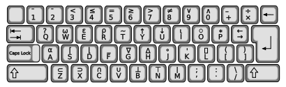
APL symbols were supported using teletypewriters with a custom keyboard layout and typeballs that could display these symbols on paper.
Not all users would have this special teletypwriter, so APL supports the standard keyboard and printer character set using transliterations for symbols. For example, the divide operator ÷ is replaced with / and the ceiling operator ⌈, which finds the maximum of its arguments, is replaced with either $MA or $CE.
The hardware used by MTS for APL is not supported on Hercules so we will need to use these transliterations when running MTS under emulation.
Prerequisites
Unlike other languages seen so far, we do need to set up APL before using it by installing it from the D5 tapes. The below method was adapted from work done by user halfmeg on the H390-MTS list.
Start with a regular D6.0 setup as described in this guide. Ensure that MTS is not running before following these steps.
Get a copy of the D5 tapes from Bitsavers and extract into a temporary directory.
Locate the files d5.0t1.aws and d5.0t2.aws under the extraction directory and copy these to the Tapes directory under your MTS install
Edit your hercules.cnf and add these lines. These tape devices are unused in the stock D6.0 install; if you have already assigned these for your own use then change the device names here and in the instructions below.
The batch instructions to restore APL from these disks is available as a card deck from my github repo on MTS languages. Download that file and copy it to Units/RDR1.txt under your Hercules install, replacing the existing file. Note that the whitespace in the first line is important, so clone the git repo or download the file as raw text.
Start up MTS as normal, including HASP. When it is running, type devinit c from the Hercules console to load the card deck. You should see the below printed on the MTS console if this worked.
00051 MTS **** Remove tape from T90B (6250 BPI)
00051 MTS **** Remove tape from T90C (6250 BPI)
The output from the batch job can be found on the printer in Hercules file Units/PTR2.txt. Examine it for any errors; you can ignore lines like You restored files saved before FEB. 22, 1988. You should see that job extracted files from the tape and set permissions appropriately.
Finally, test that it works by logging into a normal user account (eg ST01) and running
$run *APL,par=sp,noball
The APL start up message should appear. Type )LIB 1 and you should see this listing of library files:
 ADVANCEDE
 APLCOURSE
 CLASS
 NEWS
 PLOTFORMA
 TYPEDRILL
 WSFNS
 EIGENVALU
 BRFNS
Type )OFF to exit APL.
When you next shutdown MTS, you can comment out the two D5.0 tapes in hercules.cnf to free up these devices for future use.
Running a program using *APL
*APL is an interactive environment where you can enter expressions and program lines. To start APL, run *APL with the parameters sp (to print spaces after each operator) and noball (to indicate we are not using the special APL typeball.
APL prompts with six leading spaces. You can enter expressions and get results back immediately, aligned in column 1.
System commands start with ). )SOURCE will read lines from a given text file and execute them. )CONTINUE will save a copy of the current workspace to a binary file which will automatically be loaded next time you start APL. )OFF will exit APL.
Hello world
As an example, here’s a simple program to print ‘Hello, world!’ five times. This uses a simple loop - there’s probably a more concise way to do this.
First, create a file called hello.apl containing the following lines:
After you enter the )SOURCE command APL will read the file but will not prompt you it has completed. Press the ATTN key to interrupt APL and return control to you. You can then enter HELLO to run the loaded program:
In the next post we’ll look at the APL language in more detail.
Further information
IBM’s APL\360 Primer is a great first read as it introduces the APL\360 system and APL language in a tutorial form. The APL\360 User’s Manual can then be consulted for more in-depth information.
A classic introduction to APL is “APL 360: An Interactive Approach” by Gillman and Rose. A copy can be found at the Software Preservation Group of the Computer History Museum.
UM Computing Center Memo 382 is a guide to the implementation of APL\360 on MTS. I recommend reading the printed copy of this memo from the above source as it includes the hand written APL symbols missing on the source copy.
In the final part of this series, let’s create a real program in PIL.
The problem
We will implement arabic to roman number conversion from Rosetta Code.
The algorithm we’re going to use is similar to the one used there for BASIC:
Have a table of all distinct roman numbers ordered by size, including the -1 variants like IV. So roman(0) = “M”, roman(1) = “CM”, roman(2) = “D” etc.
Have another table with the same indices for their arabic equivalents. arabic(0) = 1000, arabic(1) = 900, arabic(2) = 500 etc.
Loop through each index. For each, if the input value is greater than the value of the arabic table at that value, accumulate the roman equivalent at the end of the output string and decrease the input value by the arabic amount. Keep doing this until the remaining input value is smaller than the arabic number.
So for input 2900 the steps would be
index 0, output -> “M”, input -> 1900
index 0, output -> “MM” , input -> 900
index 1, output -> “MMCM”, input -> 0 and end
The solution
As PIL is an interpreted language I’ll show a lightly reformatted transcript of my session as I build up the program in separate parts (and make mistakes along the way). Let’s get started!
First we need to set up the tables for arabic numbers in part 1. I will use the number command so that PIL prompts me with line numbers followed by an underscore automatically.
The unnumber command exits numbered line prompting mode. It needs to be prefixed with $ to be executed immediately rather than be entered as part of the program.
Let’s run that immediately so we can check it looks correct
Let’s now make the main loop to convert the number. We’ll do it in three parts, first the loop over the indices. I put in some comments fir the function.
*number 5, 0.01
&*5.0 _* Main entry point to arabic -> roman converter
&*5.01 _* Input: a (arabic number to convert)
&*5.02 _* Output: r (roman number equivalent of a)
&*5.03 _for i = 0 to 12: do part 6
&*5.04 _done
&*5.05 _$unnumber
Next, the loop for each arabic number. We can use a for with a dummy variable and the while controlling how often it is run.
*number 6, 0.01
&*6.0 _for j = 0 while a >= arabic(i): do part 7
&*6.01 _done
&*6.02 _$unnumber
Finally, in part 7 build up the roman number string and decrease the arabic number.
*number 7, 0.01
&*7.0 _r = r + roman(i)
&*7.01 _a = a - arabic(i)
&*7.02 _done
&*7.03 _$unnumber
Let’s see what these look like now.
*type part 5, part 6, part 7

  5.0    * Main entry point to arabic -> roman converter
  5.01   * Input: a (arabic number to convert)
  5.02   * Output: r (roman number equivalent of a)
  5.03   for i = 0 to 12: do part 6
  5.04   done


  6.0    for j = 0 while a >= arabic(i): do part 7
  6.01   done


  7.0    r = r + roman(i)
  7.01   a = a - arabic(i)
  7.02   done
Trying it out
We can set up the input number in a then call part 5 to convert. The output should go into r.
*a = 13
*do part 5
  Error at step 7.0: r = ?
Ah, r is not initialised so cannot be appended to. We can patch part 5 and try again.
*5.025 r = ""
*do part 5
*type r
  r = "XIII"
*type a
  a =  0.0
Great! There is a side effect though, the input value in a is wiped out as PIL does not have local variables.
Thinking about it, we are relying on the tables being initialised when we run part 5. We should really make it stand-alone by calling part 1 and 2 first.
*5.026 do part 1
*5.027 do part 2
Making it interactive
We should have a way to prompt for a number and then display the conversion.
*number 10, 0.01
&*10.0 _demand a
&*10.01 _do part 5
&*10.02 _type r
&*10.03 _$unnumber

*do part 10
& a = ? _1992
  r = "MCMXCII"
Unit tests!
It may be anachronistic, but we should have some unit tests to see if the conversion works. First let’s define a unit test handler in part 20 that takes the arabic number in a, the expected result in rExpected and then checks this matches.
*number 20, 0.01
&*20.0 _do part 5
&*20.01 _if r = rExpected, then type "OK", r; else type "ERROR', r, rExpected
  Error at step 20.01: SYMBOLIC NAME TOO LONG
&*20.02 _if r = re, then type "OK", r; else type "ERROR", r, re
&*20.03 _done
&*20.04 _$unnumber
rExpected is too long for a variable number so we use a shorter name instead, re.
Let’s test the tester out.
*re = "XLII"
*a = 42
*do part 20
  Error at step 20.01: SYMBOLIC NAME TOO LONG
Ah, the bad line is still there, so delete that and try again.
*delete step 20.01
*do part 20
  ERROR
  r = ""
  re = "XLII"
Wait, that’s not right, why is the output in r blank?
 *type r
  r = ""
 *type a
  a =  0.0
Oh OK, a is clobbered. Let’s set it up again.
*a = 42
*do part 5
*type r
  r = "XLII"
*do step 20.02
  OK
  r = "XLII"
*do step 20.02
  OK
  r = "XLII"
*type part 20

  20.0    do part 5
  20.02   if r = re, then type "OK", r; else type "ERROR", r, re
  20.03   done

*a = 42
*re = "XLII"
*do part 20
  OK
  r = "XLII"
That fixed it. Try the error case.
*a = 42
*re = "XXX"
*do part 20
  ERROR
  r = "XLII"
  re = "XXX"
*do part 21
  OK
  r = "MMIX"
  OK
  r = "MDCLXVI"
  OK
  r = "MMMDCCCLXXXVIII"
All green. However we did not test all cases such as zero, negative numbers, non-integral numbers etc.
Save and load
To confirm the program is all done and we are not relying on anything in the environment, save it to disk, quit and come back into PIL and try re-running.
*create "roman.pil"
  FILE "ROMAN.PIL" IS CREATED
*save as "roman.pil", all parts
  SAVE COMPLETED
*stop
# Execution terminated   18:51:16  T=0.279

# $run *pil
# Execution begins   18:51:37
  PIL/2: Ready
*load "roman.pil"
*do part 10
& a = ?  _42
  r = "XLII"
*do part 21
  OK
  r = "MMIX"
  OK
  r = "MDCLXVI"
  OK
  r = "MMMDCCCLXXXVIII"
*stop
The complete listing
*type all parts

  1.0    arabic(0) = 1000
  1.01   arabic(1) = 900
  1.02   arabic(2) = 500
  1.03   arabic(3) = 400
  1.04   arabic(4) = 100
  1.05   arabic(5) = 90
  1.06   arabic(6) = 50
  1.07   arabic(7) = 40
  1.08   arabic(8) = 10
  1.09   arabic(9) = 9
  1.1    arabic(10) = 5
  1.11   arabic(11) = 4
  1.12   arabic(12) = 1

  2.0    roman(0) = "M"
  2.01   roman(1) = "CM"
  2.02   roman(2) = "D"
  2.03   roman(3) = "CD"
  2.04   roman(4) = "C"
  2.05   roman(5) = "XC"
  2.06   roman(6) = "L"
  2.07   roman(7) = "XL"
  2.08   roman(8) = "X"
  2.09   roman(9) = "IX"
  2.1    roman(10) = "V"
  2.11   roman(11) = "IV"
  2.12   roman(12) = "I"

  5.0    * Main entry point to arabic -> roman converter
  5.01   * Input: a (arabic number to convert)
  5.02   * Output: r (roman number equivalent of a)
  5.025  r = ""
  5.026  do part 1
  5.027  do part 2
  5.03   for i = 0 to 12: do part 6
  5.04   done

  6.0    for j = 0 while a >= arabic(i): do part 7
  6.01   done

  7.0    r = r + roman(i)
  7.01   a = a - arabic(i)
  7.02   done

  10.0    demand a
  10.01   do part 5
  10.02   type r

  20.0    do part 5
  20.02   if r = re, then type "OK", r; else type "ERROR", r, re
  20.03   done

  21.0    a = 2009
  21.01   re = "MMIX"
  21.02   do part 20
  21.03   a = 1666
  21.04   re = "MDCLXVI"
  21.05   do part 20
  21.06   a = 3888
  21.07   re = "MMMDCCCLXXXVIII"
  21.08   do part 20
  21.09   done
Final thoughts
JOSS is a simple but well designed language - it’s easy to pick up, has a carefully chosen set of features and does the job it’s supposed to do well. Compared to BASIC it seems much more intuitive as a simple language for non-specialists who want to get numeric calculations done quickly. The lack of functions and local variables, plus the heavily interactive nature of the language makes it harder to write larger programs, but given the first version was running in 1963 it’s quite an impressive feat of engineering.
PIL, the version of JOSS implemented on MTS, improves the usability of the original language, eg by not requiring a period at the end of each statement. There is enough integration with the operating system to make it usable. It would be interesting to know what type of use it got at UM.
Several languages were inspired by JOSS, including FOCAL on PDP-8s. It’s also one of the influences on MUMPS, which is still in use today.
Further information
Full source code for this program can be found on github.
In the last post we saw some of the history of PIL and how to run it on MTS. We’ll now take a closer look at the features of PIL. Examples shown can be entered directly into PIL after starting it with $run *pil.
Direct mode
PIL starts up in direct mode, where statements entered are immediately executed when you press RETURN. * is used by PIL as the prompt to enter input. You can use the TYPE statement and simple arithmetic expressions to make PIL act as a calculator:
* type 22 * 2
  22 * 2 =  44.0
* type 2 ** 16
  2 ** 16 =  65536.0
On MTS, PIL is case-insensitive for keywords and lines can optionally end with a period. Errors are immediately reported, usually starting with Eh?.
* TYPE 2+2.
  2+2 =  4.0
* TYPE
  Eh? IMPROPERLY FORMED STATEMENT
If the last character entered on the line is - then input will continue on the next line before it is executed. The prompt will change to & to show this continuation. * at the start of line can be used to make comments.
Variables can be introduced by the optional keyword SET followed by a variable name and an assignment.
* set a = 2
* b = 3
* type a, b, a+b
  a =  2.0
  b =  3.0
  a+b =  5.0
PIL understands three types: numerical, which are stored as floating point values, character strings and Boolean values.
* a = 1 / 3
* b = "PIL"
* c = The True
* type a, b, c
  a =  0.3333333
  b = "PIL"
  c = The True
Booleans constants are ‘The True’ or ‘The False’ - something I’ve not seen in any other language. Strings can be up to 255 characters long and can be entered with single or double quotes as delimiters. Floats have 7 digits of precision and can be entered with exponential notation. Volume 12 mentions type 9.999999e64 as the maximum value but on the version I’m running it seems 62 is the maximum exponent.
* type 9.999999e62
  9.999999e62 =  9.999999E+62
* type 9.999999e63
  Eh? EXPONENT OUT OF RANGE
Variable names are up to 8 characters long, are case sensitive and are distinguished from keywords, as this silly example shows.
* set set = 1
* set SET = 2
* type set, SET
  set =  1.0
  SET =  2.0
Arrays are allowed with any number of dimensions, though once set the number of dimensions cannot be changed.
Arithmetic expressions work mostly as expected. The absolute value can be taken by surrounding an expression with |; exponentiation is done with **. Functions for arithmetic operations such as square root, cosine, log etc generally have a short and long form and do not need parentheses unless needed to resolve ambiguities.
* type 1 + |-41|
  1 + |-41| =  42.0
* type the square root of 9
  the square root of 9 =  3.0
* type sqrt of 16
  sqrt of 16 =  4.0
* type sqrt of 25+1
  sqrt of 25+1 =  6.0
* type sqrt of (25+1)
  sqrt of (25+1) =  5.09902
There are functions for min/max, random numbers and extracting parts of a number, as well as special functions to get time (in 300ths of seconds since midnight), date, cpu/elapsed time and storage used.
* type the min of (1,2,3)
  the min of (1,2,3) =  1.0
* type the time, the date, the elapsed time, the cpu time
  the time =  1.963908E+07
  the date =  17133.0
  the elapsed time =  7.819461E+07
  the cpu time =  464.0
* type the total size, the size
  the total size =  188.0
  the size =  165.0
Boolean functions are similar to other languages, with # standing in for logical or.
* type 2 >= 3
  2 >= 3 = The False
* type 2 $lt 3
  2 $lt 3 = The True
* type the true # the false
  the true # the false = The True
* type the true & the false
  the true & the false = The False
Character expressions include length, case conversion, comparison and extraction.
* type the l of "abc"
  the l of "abc" =  3.0
* type the upper of "abC"
  the upper of "abC" = "ABC"
* type the first 3 characters of "abcde"
  the first 3 characters of "abcde" = "abc"
* type 2 $fc "abcde" + "X" + 1 $lc "abcde"
  2 $fc "abcde" + "X" + 1 $lc "abcde" = "abXe"
* type "aaa" > "AAA"
  "aaa" > "AAA" = The False
Finally, the type of an expression can be found and run time evaluation performed.
* type the mode of 42, the mode of the true, the mode of "abc"
  the mode of 42 =  1.0
  the mode of the true =  2.0
  the mode of "abc" =  3.0
* type the value of "2*21"
  the value of "2*21" =  42.0
Control flow
There’s an IF statement with an optional ELSE clause. The IF and ELSE can be omitted but the punctuation is required.
* if 1 < 2, then type 'yes'; else type 'no'
  yes
* if 1 > 2, type 'yes'; type 'no'
  no
For loops have a range or an increment and an optional clause to terminate.
* for i = 1 to 5: type i ** 2
  i ** 2 =  1.0
  i ** 2 =  4.0
  i ** 2 =  9.0
  i ** 2 =  16.0
  i ** 2 =  25.0
* for i = 1 by 2 to 10: type i ** 2
  i ** 2 =  1.0
  i ** 2 =  9.0
  i ** 2 =  25.0
  i ** 2 =  49.0
  i ** 2 =  81.0
* for i = 1 by 2 while i < 20: type i
  i =  1.0
  i =  3.0
  i =  5.0
  i =  7.0
  i =  9.0
  i =  11.0
  i =  13.0
  i =  15.0
  i =  17.0
  i =  19.0
Indirect mode
Lines entered that start with a number are treated as stored instructions, broken down by part and step, that can be run later. Here we define a program in part 1 consisting of four steps.
* 1.0 i = 5
* 1.1 type i
* 1.2 i = i * i
* 1.3 type i
This can then be run with DO, which will execute all steps in a part.
* do part 1
  i =  5.0
  i =  25.0
Variables set in a program remain after execution is completed and it is possible to run a single step at a time.
* type i
  i =  25.0
* do step 1.2
* do step 1.3
  i =  625.0
Steps can call other parts with DO: execution will resume after the part is finished. It’s also possible to transfer execution with TO which will not return. DONE will return from the current part.
* type part 2, part 3

  2.0    i = 3
  2.1    do step 3
  2.2    i = 5
  2.3    do step 3
  2.4    i = 7
  2.5    to step 3
  2.6    type 'not reached'


  3.0    type i
  3.1    done
  3.2    type 'also not reached'

* do part 2
  i =  3.0
  i =  5.0
  i =  7.0
The above also shows it is possible to list out programs with TYPE PART. You can see all entered parts with TYPE ALL PARTS. With TYPE ALL STUFF you will see all variables and parts defined.
DELETE can be used to remove a step or a variable definition.
I/O and system access
We’ve seen TYPE used to display variables. You can prompt for a value to be entered with DEMAND
* delete part 1
* 1.0 demand i
* 1.1 i = i * 10
* 1.2 type i
* do part 1
 i = ?_ 3
  i =  30.0
There is also a formatting facility for input and output that is covered in the manual.
Programs can be saved to disk for future list with SAVE. This takes a file name (which must already exist) and what to save. For example:
save as 'x.pil', all stuff
will save all parts and variables to x.pil. File format is plain text so it can be edited outside of PIL if needed. LOAD 'x.pil' will then load the file back into PIL.
The implementation of PIL on MTS includes access to system facilities such as file creation and device access. For example, CREATE 'x.pil' will create a new file.
In the next post we’ll see how to construct a larger PIL program.
Further information
MTS volume 12 has a complete reference to PIL as implemented on MTS.
If you can find a copy of the book ‘History of Programming Languages’, edited by Richard Wexelblat, this has a great section about JOSS talking about its design principles.